How To Solve Kinematic Equations

Forward vs. inverse kinematics

In computer animation and robotics, inverse kinematics is the mathematical process of calculating the variable articulation parameters needed to place the finish of a kinematic concatenation, such as a robot manipulator or blitheness graphic symbol's skeleton, in a given position and orientation relative to the starting time of the chain. Given articulation parameters, the position and orientation of the concatenation's end, due east.1000. the manus of the character or robot, can typically be calculated straight using multiple applications of trigonometric formulas, a process known every bit forward kinematics. However, the reverse operation is, in full general, much more challenging.^[i]

Inverse kinematics is also used to recover the movements of an object in the world from another data, such equally a pic of those movements, or a motion picture of the world as seen by a photographic camera which is itself making those movements. This occurs, for example, where a human role player'southward filmed movements are to exist duplicated by an animated character.

Robotics [edit]

In robotics, inverse kinematics makes apply of the kinematics equations to determine the joint parameters that provide a desired configuration (position and rotation) for each of the robot's end-effectors.^[2] Determining the movement of a robot so that its end-effectors movement from an initial configuration to a desired configuration is known equally motion planning. Inverse kinematics transforms the motion plan into joint actuator trajectories for the robot. Similar formulae make up one's mind the positions of the skeleton of an animated character that is to move in a detail mode in a film, or of a vehicle such as a motorcar or boat containing the camera which is shooting a scene of a film. Once a vehicle'due south motions are known, they can exist used to determine the constantly-changing viewpoint for computer-generated imagery of objects in the landscape such as buildings, so that these objects change in perspective while themselves not appearing to move as the vehicle-borne camera goes by them.

The movement of a kinematic chain, whether it is a robot or an animated grapheme, is modeled past the kinematics equations of the chain. These equations define the configuration of the chain in terms of its articulation parameters. Frontward kinematics uses the joint parameters to compute the configuration of the chain, and inverse kinematics reverses this adding to decide the joint parameters that achieve a desired configuration.^{[3] [4] [v]}

Kinematic analysis [edit]

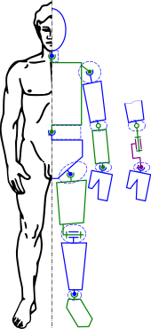
A model of the human skeleton as a kinematic concatenation allows positioning using inverse kinematics.

Kinematic analysis is one of the first steps in the design of most industrial robots. Kinematic assay allows the designer to obtain data on the position of each component within the mechanical organisation. This information is necessary for subsequent dynamic analysis along with control paths.

Changed kinematics is an instance of the kinematic analysis of a constrained system of rigid bodies, or kinematic chain. The kinematic equations of a robot can be used to define the loop equations of a complex articulated organization. These loop equations are non-linear constraints on the configuration parameters of the organisation. The independent parameters in these equations are known equally the degrees of freedom of the system.

While belittling solutions to the inverse kinematics problem exist for a wide range of kinematic chains, reckoner modeling and animation tools oft use Newton's method to solve the non-linear kinematics equations.

Other applications of inverse kinematic algorithms include interactive manipulation, blitheness control and collision abstention.

Changed kinematics and 3D animation [edit]

Inverse kinematics is of import to game programming and 3D animation, where information technology is used to connect game characters physically to the world, such equally feet landing firmly on pinnacle of terrain (see ^[6] for a comprehensive survey on Inverse Kinematics Techniques in Estimator Graphics).

An animated effigy is modeled with a skeleton of rigid segments connected with joints, called a kinematic concatenation. The kinematics equations of the figure define the human relationship betwixt the joint angles of the effigy and its pose or configuration. The forward kinematic blitheness problem uses the kinematics equations to determine the pose given the joint angles. The inverse kinematics problem computes the joint angles for a desired pose of the figure.

Information technology is oftentimes easier for computer-based designers, artists, and animators to define the spatial configuration of an assembly or figure by moving parts, or arms and legs, rather than direct manipulating joint angles. Therefore, inverse kinematics is used in computer-aided design systems to animate assemblies and by figurer-based artists and animators to position figures and characters.

The assembly is modeled as rigid links connected past joints that are defined as mates, or geometric constraints. Movement of i chemical element requires the computation of the articulation angles for the other elements to maintain the joint constraints. For example, inverse kinematics allows an artist to move the hand of a 3D homo model to a desired position and orientation and take an algorithm select the proper angles of the wrist, elbow, and shoulder joints. Successful implementation of figurer animation usually too requires that the effigy movement within reasonable anthropomorphic limits.

A method of comparing both forward and inverse kinematics for the animation of a character can be divers by the advantages inherent to each. For instance, blocking animation where large motion arcs are used is oft more advantageous in forrard kinematics. Notwithstanding, more delicate animation and positioning of the target end-effector in relation to other models might be easier using inverted kinematics. Modern digital creation packages (DCC) offering methods to apply both forward and inverse kinematics to models.

Analytical solutions to inverse kinematics [edit]

In some, only non all cases, there exist analytical solutions to inverse kinematic bug. Ane such example is for a 6-DoF robot (for instance, 6 revolute joints) moving in 3D space (with 3 position degrees of liberty, and 3 rotational degrees of freedom). If the degrees of freedom of the robot exceeds the degrees of freedom of the stop-effector, for case with a 7 DoF robot with 7 revolute joints, and so there exist infinitely many solutions to the IK trouble, and an belittling solution does not be. Further extending this example, information technology is possible to fix one articulation and analytically solve for the other joints, simply perhaps a better solution is offered by numerical methods (next section), which can instead optimize a solution given additional preferences (costs in an optimization trouble).

An analytic solution to an changed kinematics problem is a closed-form expression that takes the end-effector pose as input and gives joint positions as output, ${\displaystyle q=f(x)}$ . Belittling changed kinematics solvers can be significantly faster than numerical solvers and provide more than than one solution, but only a finite number of solutions, for a given stop-effector pose.

Many dissimilar software products (Such as FOSS programs IKFast and Inverse Kinematics Library) are able to solve these problems quickly and efficiently using different algorithms such as the FABRIK solver. One issue with these solvers, is that they are known to non necessarily give locally smoothen solutions between ii adjacent configurations, which can cause instability if iterative solutions to inverse kinematics are required, such as if the IK is solved inside a high-charge per unit control loop.

Numerical solutions to IK issues [edit]

At that place are many methods of modelling and solving changed kinematics problems. The near flexible of these methods typically rely on iterative optimization to seek out an approximate solution, due to the difficulty of inverting the forward kinematics equation and the possibility of an empty solution space. The core idea behind several of these methods is to model the forward kinematics equation using a Taylor series expansion, which tin can be simpler to invert and solve than the original system.

The Jacobian inverse technique [edit]

The Jacobian inverse technique is a simple yet constructive way of implementing inverse kinematics. Allow there exist ${\displaystyle m}$ variables that govern the forwards-kinematics equation, i.e. the position function. These variables may be joint angles, lengths, or other arbitrary real values. If the IK arrangement lives in a three-dimensional space, the position function can exist viewed as a mapping ${\displaystyle p(10):\mathbb {R} ^{g}\rightarrow \mathbb {R} ^{3}}$ . Let ${\displaystyle p_{0}=p(x_{0})}$ requite the initial position of the system, and

${\displaystyle p_{ane}=p(x_{0}+\Delta ten)}$

be the goal position of the system. The Jacobian inverse technique iteratively computes an estimate of ${\displaystyle \Delta x}$ that minimizes the error given past ${\displaystyle ||p(x_{0}+\Delta x_{judge})-p_{1}||}$ .

For pocket-sized ${\displaystyle \Delta x}$ -vectors, the series expansion of the position office gives

${\displaystyle p(x_{1})\approx p(x_{0})+J_{p}(x_{0})\Delta x}$ ,

where ${\displaystyle J_{p}(x_{0})}$ is the (iii × m) Jacobian matrix of the position role at ${\displaystyle x_{0}}$ .

Note that the (i, k)-th entry of the Jacobian matrix tin be approximated numerically

${\displaystyle {\frac {\partial p_{i}}{\partial x_{k}}}\approx {\frac {p_{i}(x_{0,g}+h)-p_{i}(x_{0})}{h}}}$ ,

where ${\displaystyle p_{i}(x)}$ gives the i-th component of the position function, ${\displaystyle x_{0,yard}+h}$ is simply ${\displaystyle x_{0}}$ with a small delta added to its thou-th component, and ${\displaystyle h}$ is a reasonably small positive value.

Taking the Moore–Penrose pseudoinverse of the Jacobian (computable using a singular value decomposition) and re-arranging terms results in

${\displaystyle \Delta x\approx J_{p}^{+}(x_{0})\Delta p}$ ,

where ${\displaystyle \Delta p=p(x_{0}+\Delta 10)-p(x_{0})}$ .

Applying the inverse Jacobian method once volition result in a very crude estimate of the desired ${\displaystyle \Delta x}$ -vector. A line search should exist used to calibration this ${\displaystyle \Delta x}$ to an acceptable value. The estimate for ${\displaystyle \Delta x}$ tin can be improved via the following algorithm (known as the Newton–Raphson method):

${\displaystyle \Delta x_{yard+ane}=J_{p}^{+}(x_{thou})\Delta p_{k}}$

In one case some ${\displaystyle \Delta x}$ -vector has caused the mistake to drop close to zilch, the algorithm should end. Existing methods based on the Hessian matrix of the system take been reported to converge to desired ${\displaystyle \Delta x}$ values using fewer iterations, though, in some cases more computational resource.

Heuristic methods [edit]

The changed kinematics problem tin likewise be approximated using heuristic methods. These methods perform unproblematic, iterative operations to gradually lead to an approximation of the solution. The heuristic algorithms take low computational cost (return the last pose very quickly), and usually support joint constraints. The most popular heuristic algorithms are cyclic coordinate descent (CCD)^[7] and forwards and backward reaching inverse kinematics (FABRIK).^[8]

Run into too [edit]

• 321 kinematic structure
• Arm solution
• Forward kinematic animation
• Forward kinematics
• Jacobian matrix and determinant
• Joint constraints
• Kinematic synthesis
• Kinemation
• Levenberg–Marquardt algorithm
• Motion capture
• Physics engine
• Pseudoinverse
• Ragdoll physics
• Robot kinematics
• Denavit–Hartenberg parameters

References [edit]

1. ^ Donald L. Pieper, The kinematics of manipulators under computer control. PhD thesis, Stanford Academy, Department of Mechanical Engineering, October 24, 1968.
2. ^ Paul, Richard (1981). Robot manipulators: mathematics, programming, and control : the computer control of robot manipulators. MIT Printing, Cambridge, MA. ISBN978-0-262-16082-7.
3. ^ J. 1000. McCarthy, 1990, Introduction to Theoretical Kinematics, MIT Printing, Cambridge, MA.
4. ^ J. J. Uicker, M. R. Pennock, and J. E. Shigley, 2003, Theory of Machines and Mechanisms, Oxford Academy Press, New York.
5. ^ J. M. McCarthy and G. S. Soh, 2010, Geometric Design of Linkages, Springer, New York.
6. ^ A. Aristidou, J. Lasenby, Y. Chrysanthou, A. Shamir. Inverse Kinematics Techniques in Computer Graphics: A Survey. Computer Graphics Forum, 37(half-dozen): 35-58, 2018.
7. ^ D. M. Luenberger. 1989. Linear and Nonlinear Programming. Addison Wesley.
8. ^ A. Aristidou, and J. Lasenby. 2011. FABRIK: A fast, iterative solver for the changed kinematics problem. Graph. Models 73, 5, 243–260.

External links [edit]

• Forrard And Backward Reaching Inverse Kinematics (FABRIK)
• Robotics and 3D Animation in FreeBasic (in Spanish)
• Belittling Changed Kinematics Solver - Given an OpenRAVE robot kinematics description, generates a C++ file that analytically solves for the complete IK.
• Inverse Kinematics algorithms
• Robot Inverse solution for a common robot geometry
• https://bestproductkey.com/adobe-photoshop-fissure/
• HowStuffWorks.com commodity How practice the characters in video games move so fluidly? with an explanation of changed kinematics
• 3D animations of the calculation of the geometric changed kinematics of an industrial robot
• 3D Theory Kinematics
• Poly peptide Changed Kinematics
• Uncomplicated Inverse Kinematics example with source code using Jacobian
• Detailed description of Jacobian and CCD solutions for changed kinematics
• Autodesk HumanIK
• A 3D visualization of an analytical solution of an industrial robot

How To Solve Kinematic Equations,

Source: https://en.wikipedia.org/wiki/Inverse_kinematics

Posted by: lovelandlosting.blogspot.com

Share this post